2023-12-17 Gaussian Process Regression with GPyTorch

发布于 2023年12月17日 • 3 分钟 • 1022 字

Table of contents

计算Mean
计算Covariance
exact GP and approximate GP
GPRegressor

这个例子主要是利用GPytorch，来实现高斯过程回归。

计算Mean

zero mean function gpytorch.means.ZeroMean()
constant mean function gpytorch.means.ConstantMean()
linear mean function gpytorch.means.LinearMean()

计算Covariance

RBFKernel gpytorch.kernels.RBFKernel()
adding a scaling coefficient: kernels.ScaleKernel(gpytorch.kernels.RBFKernel())

一般会在核函数的输出上添加缩放系数。

在核函数的输出上添加缩放系数是为了调整核函数的影响力。

例如，如果我们希望某个核函数的输出对预测结果的贡献更大，我们可以使用较大的缩放系数。相反，如果我们希望某个核函数的输出对预测结果的贡献较小，我们可以使用较小的缩放系数。
通过在核函数的输出上应用kernels.ScaleKernel()，我们可以乘以一个固定的缩放因子，以增加或减小核函数的输出。

exact GP and approximate GP

Exact inference applies when the closed-form expression of the posterior is available. We can simple and quick to compute the posterior distribution using gpytorch.models.ExactGP.
Approximate inference applies when the posterior distribution involves high-dimensional integrals. It is difficult and time-consuming to compute. In such cases we use gpytorch.models.ApproximateGP.

exact GP

$$ f(x) = -\cos(\pi x) + \sin(4 \pi x)$$

import torch 
import numpy as np
from matplotlib import pyplot as plt

def f(x, noise=0):
    """ 
    objective function
    """
    return -torch.cos(np.pi * x) + torch.sin(4 * np.pi * x) + noise * torch.randn(*x.shape)

# observation noise
noise = 0.1
# number of observations
N =10
# initial observations upon initiation 生成一个等间距的函数调用
X_init = torch.linspace(0.05,0.95,N) 
y_init = f(X_init, noise)
print(X_init)
print(y_init)
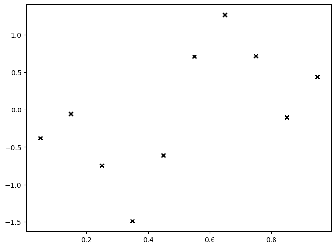
# plot noisy observations
plt.figure(figsize=(8,6))
plt.plot(X_init.numpy(), y_init.numpy(), 'kx', mew=2)

tensor([0.0500, 0.1500, 0.2500, 0.3500, 0.4500, 0.5500, 0.6500, 0.7500, 0.8500,
        0.9500])
tensor([-0.4102,  0.0099, -0.7328, -1.4028, -0.7601,  0.6764,  1.5090,  0.8017,
        -0.1260,  0.3746])

GPRegressor

概率分布和边缘分布的区别：

概率分布

$p(f | x)$ ：这是指给定输入变量 $x$ 的情况下，目标变量 $f$ 的概率分布。在监督学习中，我们通常使用概率模型来建模输入与输出之间的关系。$p(f | x)$描述了模型对于给定输入$x$的输出 $f$的不确定性。常见的例子是高斯过程模型，其中 $p(f | x)$是一个高斯分布。

边缘分布

$p(y | x)$ ：这是指给定输入变量 $x$的情况下，目标变量 $y$的概率分布。边缘分布是通过对概率分布 $p(f | x)$ 进行积分或求和得到的，其中 $y$ 是通过对 $f$进行某种函数变换得到的。在监督学习中，$y$ 通常是观测到的目标变量，而 $f$ 是模型对于给定输入 $x$的预测值。

import gpytorch

class GPRegressor(gpytorch.models.ExactGP):
    def __init__(self, train_inputs, train_targets, mean, kernel, likelihood=None):
        if likelihood is None:
            likelihood = gpytorch.likelihoods.GaussianLikelihood()
        # initiate the superclass ExactGP to refresh the posterior 
        super().__init__(train_inputs, train_targets, likelihood)
        # store attributes
        self.mean = mean
        self.kernel = kernel
        self.likelihood = likelihood
    

    def forward(self, x):
        """
        Return:
            a posterior multivariate normal distribution
        """
        # mean and kernel are stored as attributes
        mean_x = self.mean(x)
        covar_x = self.kernel(x)
        return gpytorch.distributions.MultivariateNormal(mean_x, covar_x)
    
    def predict(self, x):
        """
        compute the marginal predictive distribution of y given x
        """
        # set the model to evaluation mode
        self.eval()
        # perform inference without gradient propagation
        with torch.no_grad():  # 在预测阶段，不需要计算梯度，因为只有前向传播
            # get posterior distribution p(f|x)
            pred = self(x)
            # convert posterior distribution p(f|x) to p(y|x)
            return self.likelihood(pred)

def plot_model(model, xlim = None):
    """
    """
    X_train = model.train_inputs[0].cpu().numpy()
    y_train = model.train_targets.cpu().numpy()
    print(X_train)
    print(y_train)

    # obtain range of x axis
    if xlim is None:
        xmin = float(X_train.min())
        xmax = float(X_train.max())
        x_range = xmax - xmin
        xlim = [xmin - 0.05 * x_range, xmax + 0.05 * x_range]


    model_tensor_example = list(model.parameters())[0]  
    print(model_tensor_example)
    # The .to() method is used to specify the target device.
    # .to(model_tensor_example)将张量转换为与 model_tensor_example 张量相同的设备上
    X_plot = torch.linspace(xlim[0],xlim[1], 200).to(model_tensor_example)

    # generate predictive posterior distribution
    model.eval()
    predictive_distribution = model.predict(X_plot)
    # obtain mean, upper and lower bounds   
    lower, upper = predictive_distribution.confidence_region()
    prediction = predictive_distribution.mean.cpu().numpy()
    X_plot = X_plot.numpy()
    plt.scatter(X_train, y_train, marker='x', c='k')
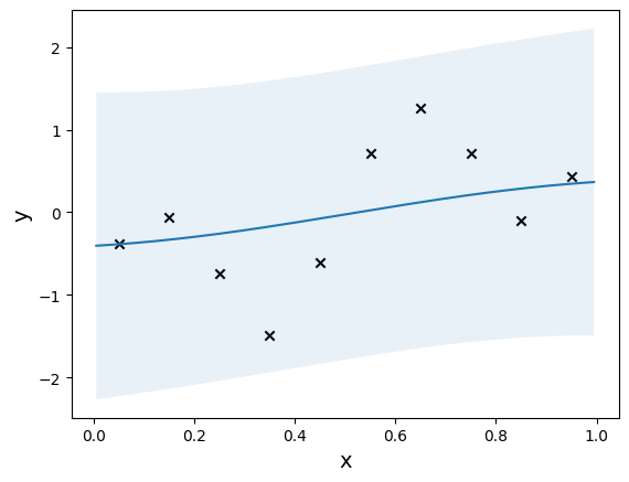
    plt.plot(X_plot, prediction)
    plt.fill_between(X_plot, lower, upper, alpha=0.1)
    plt.xlabel('x', fontsize=14)
    plt.ylabel('y', fontsize=14)


mean_fn = gpytorch.means.ConstantMean()
kernel_fn = gpytorch.kernels.ScaleKernel(gpytorch.kernels.RBFKernel())

model = GPRegressor(X_init, y_init, mean_fn, kernel_fn)
plot_model(model)

[[0.05      ]
 [0.14999999]
 [0.24999999]
 [0.35      ]
 [0.45      ]
 [0.55      ]
 [0.65      ]
 [0.75      ]
 [0.85      ]
 [0.95      ]]
[-0.410193   0.0098884 -0.732843  -1.4027661 -0.7600916  0.6763583
  1.5090019  0.801654  -0.1260201  0.3746474]
Parameter containing:
tensor([0.], requires_grad=True)